1 Figure 1

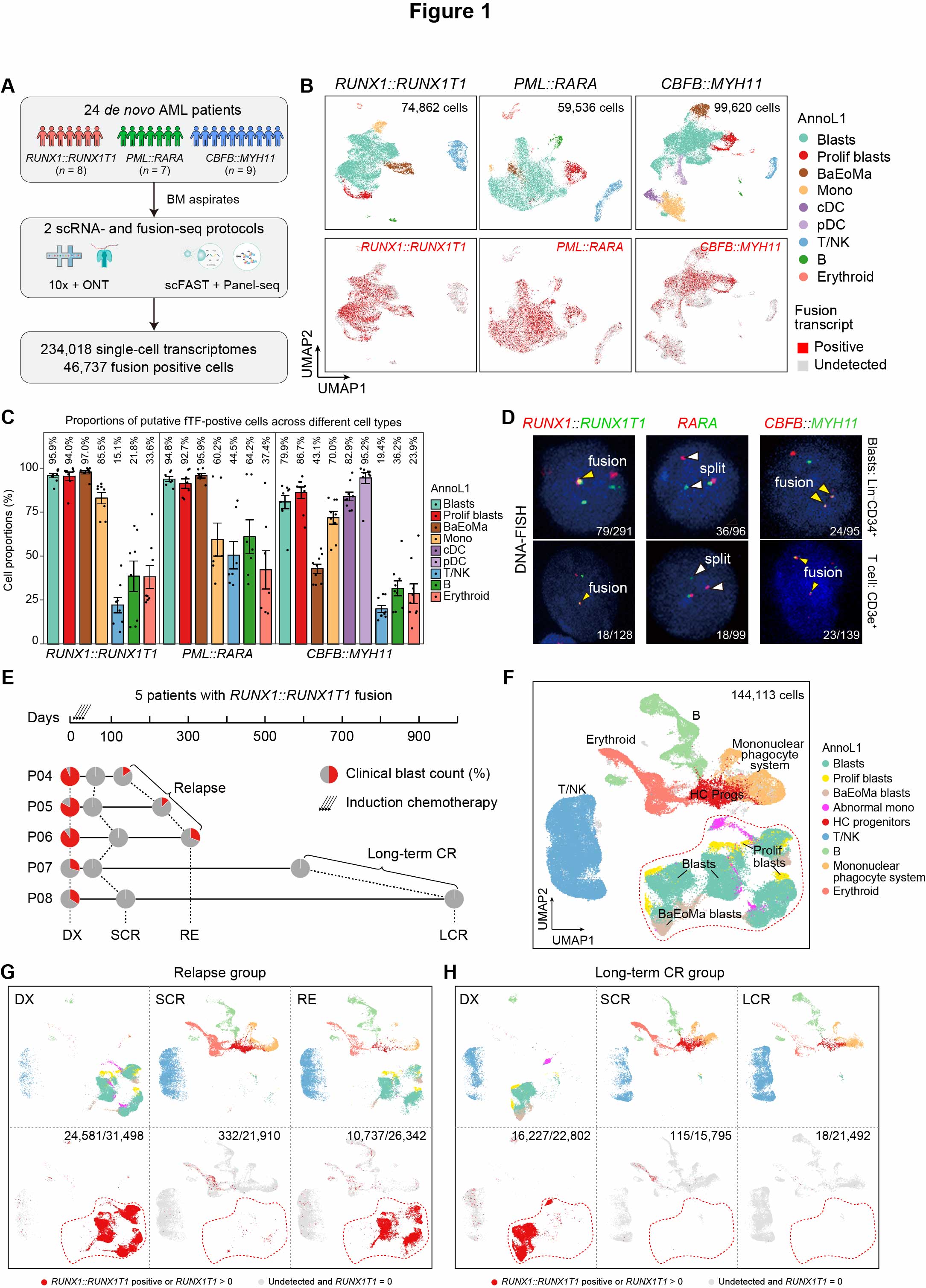Fig. 1. scRNA-seq profiling and detection of fusion gene transcripts in AML subtypes

(A) Schematic representation of the study design.
(B) Top panel: UMAP visualization of nine broad cell types from various AML subtypes. Colors indicate major cell types. Bottom panel: UMAP visualization of cells expressing RUNX1::RUNX1T1, PML::RARA, or CBFB::MYH11, where red and grey dots indicate fusion transcript-positive and fusion transcript undetected cells, respectively.
(C) Percentage of putative fTF⁺ cells (defined by either direct fTF transcript detection or aberrant gene expression signature) in each major cell type across the RUNX1::RUNX1T1 (left), PML::RARA (middle), and CBFB::MYH11 (right) AML subtypes. Data are presented as mean ± standard error of mean (SEM).
(D) Representative DNA-FISH confocal images. Dual probes detect RUNX1::RUNX1T1 and CBFB::MYH11 (yellow arrowheads indicate fusion genes), while split probes identify PML::RARA (white arrowheads indicate the split of two RARA gene portions). Leukemic blasts and T cells were sorted as follows: Lin^-CD34⁺CD117⁺ for RUNX1::RUNX1T1 and CBFB::MYH11 blasts, Lin^-CD34^-CD117⁺ for PML::RARA blast; CD3e⁺ for T lymphocytes in all AML subtypes.
(E) Overview of serially collected BM aspirates from five RUNX1::RUNX1T1 AML patients. Pie charts illustrate the clinical blast count for each sample.
(F) UMAP visualization of nine broad cell types from RUNX1::RUNX1T1 AML longitudinal samples. Grey indicates low-quality cells. The red dashed box outlines the blast population.
(G-H) Top panel: UMAP distribution of the RUNX1::RUNX1T1 AML relapse group (G) and long-term CR group (H) at different stages, with cell types color-coded based on panel F annotations. Bottom panel: UMAP plots showing cells expressing RUNX1::RUNX1T1 or truncated RUNX1T expression > 0 at these stages, highlighting the distribution of fusion transcript-positive cells in the relapse group (G) and long-term CR group (H). Red dots indicate RUNX1::RUNX1T1⁺ cells or those with RUNX1T1 expression > 0; grey dots represent cells with no fusion transcripts and RUNX1T1 expression = 0. The number before the slash indicates putative fTF⁺ cells, and the number after the slash denotes the total cell count. Low-quality cells were excluded for clarity.

1.1 (B) UMAP distribution across AML subtypes

anno_color <- c("#73C8B4", "#E31A1C", "#A65628", "#FDBF6F", "#9970AB", "#C2A5CF", "#6BAED6", "#33A02C", "#FB8072")
anno_name <- c("Progs", "Progs_Prolif", "Progs_BaEoMa", "Mono", "cDC", "pDC", "T.NK", "B", "Erythroid")
names(anno_color) <- anno_name

scAE.anno <- read_rds(paste0(in_dir, "Table1.3.scAE_harmony.anno.rds"))
scAPL.anno <- read_rds(paste0(in_dir, "Table1.3.scAPL_harmony.anno.rds"))
scCM.anno <- read_rds(paste0(in_dir, "Table1.3.scCM_harmony.anno.rds"))


## visualization
p1_1 <- DimPlot(scAE.anno, reduction = "umap", group.by = "annoL1", 
                label = F, repel = F, raster = T, cols = anno_color, pt.size = 0.4) + labs(title = "M2")
p2_1 <- DimPlot(scAPL.anno, reduction = "umap", group.by = "annoL1",
                label = F, repel = F, raster = T, cols = anno_color, pt.size = 0.4) + labs(title = "M3")
p3_1 <- DimPlot(scCM.anno, reduction = "umap", group.by = "annoL1",
                label = F, repel = F, raster = T, cols = anno_color, pt.size = 0.4) + labs(title = "M4")

p1_2 <- DimPlot(scAE.anno, reduction = "umap", group.by = "fus_group", label = F, repel = T, order = T, raster = T,
                pt.size = 0.01, na.value = "#D9D9D9", cols = c("#E41A1C", "#D9D9D9")) + labs(title = "M2")
p2_2 <- DimPlot(scAPL.anno, reduction = "umap", group.by = "fus_group", label = F, repel = T, order = T, raster = T,
                pt.size = 0.01, na.value = "#D9D9D9", cols = c("#E41A1C", "#D9D9D9")) + labs(title = "M3")
p3_2 <- DimPlot(scCM.anno, reduction = "umap", group.by = "fus_group", label = F, repel = T, order = T, raster = T,
                pt.size = 0.01, na.value = "#D9D9D9", cols = c("#E41A1C", "#D9D9D9")) + labs(title = "M4")


pdf(paste0(out_dir, "Fig1B.pdf"), width = 9, height = 5)
p1_1 + p2_1 + p3_1 + p1_2 + p2_2 + p3_2 + plot_layout(ncol = 3, guides = "collect")
dev.off()

1.2 (C) Distribution of putative fTF-expressing cells

g_list <- c("M2AE", "M3PR", "M4CM")
annoL1_name <- c("Progs", "Progs_Prolif", "Progs_BaEoMa", "Mono", "cDC", "pDC", "T.NK", "B", "Erythroid")
annoL1_color <- c("#73C8B4", "#E31A1C", "#A65628", "#FDBF6F", "#9970AB", "#C2A5CF", "#6BAED6", "#33A02C", "#FB8072")
names(annoL1_color) <- annoL1_name

mydata <- read.xlsx(paste0(in_dir, "Fig1.6.1.SS.pred_fus_Freq_inSubCluster.xlsx"), sheet = 4)[, 26:50] %>%
  gather("SampleID", "Value", -annoL1) %>% 
  dplyr::rename("seurat_clusters" = "annoL1") %>%
  left_join(., my_df) %>%
  mutate(Type = factor(Type, g_list)) %>%
  mutate(Value = Value * 100) %>%
  filter(!is.na(Value)) %>%
  mutate(seurat_clusters = factor(seurat_clusters, levels = annoL1_name))

df <- mydata %>% group_by(Type, seurat_clusters) %>% summarise(mean = mean(Value)) %>%
  left_join(., mydata %>% group_by(Type, seurat_clusters) %>% summarise(sd = std.error(Value)))

data <- mydata %>% 
    left_join(., df, by = c("seurat_clusters" = "seurat_clusters", "Type" = "Type"))

pdf(paste0(out_dir, "Fig1C.pdf"), width = 9, height = 5)
ggplot() + 
      geom_bar(data = data, aes_string(x = "seurat_clusters", y = "mean", fill = "seurat_clusters"), 
               stat = "identity", color = "black", position = position_dodge(), width = 0.7) + 
      geom_errorbar(data = data, aes(x = seurat_clusters, y = mean, fill = seurat_clusters, 
                                     ymin = mean - sd, ymax = mean + sd), width = 0.5, position = position_dodge(0.05)) + 
      geom_jitter(data = data, aes_string(x = "seurat_clusters", y = "Value", fill = "seurat_clusters"), size = 0.5, width = 0.3) +
      scale_fill_manual(values = annoL1_color) +
      scale_y_continuous(expand = expansion(mult = c(0, 0.1))) +
      labs(x = "", y = "Percentage (%)", fill = "") + ggthemes::theme_few(base_size = 12) +
      theme(axis.text.x = element_text(angle = 90, hjust = 1, vjust = 0.5), 
            plot.title = element_text(hjust = 0.5, size = 10), legend.position = "right") + 
      facet_grid(. ~ Type, scales = "free", space = "free", drop = T)
dev.off()

1.3 (F) UMAP by annoL1 in RUNX1::RUNX1T1 AML longitudinal samples

scAE.anno <- read_rds(paste0(in_dir, "Table1.3.scAE_anno.rds"))

annoL1_color <- c("#73C8B4", "#FFEA00", "#DBBBA9", "#FF40FF", "#E31A1C", "#6BAED6", "#A1D99B", "#FDBF6F", "#FB8072", "#D9D9D9")
annoL1_name <- c("Progs", "Progs_Prolif", "Progs_BaEoMa", "Mono1", "HC_Pros", "T.NK", "B", "Myeloid", "Erythroid", "LowQual")
names(annoL1_color) <- annoL1_name

p1 <- DimPlot(scAE.anno, reduction = "umap", group.by = "annoL1", 
        label = T, repel = T, raster = T, cols = annoL1_color, pt.size = 0.5)

pdf(paste0(out_dir, "Fig1F.pdf"), width = 12, height = 4.5)
p1
dev.off()

1.4 (G-H) UMAP by stages in RUNX1::RUNX1T1 AML longitudinal samples

scAE.anno.sub <- scAE.anno %>% subset(annoL1 != "LowQual")

annoL1_color <- annoL1_color[1:9]

pdf(paste0(out_dir, "Fig1G-H_1.pdf"), width = 13.5, height = 8)
DimPlot(scAE.anno.sub, reduction = "umap", split.by = "group", group.by = "annoL2", cols = annoL2_color, 
        label = F, repel = T, raster = T, pt.size = 0.5, ncol = 3)
dev.off()


scAE.anno.sub2 <- scAE.anno.sub
scAE.anno.sub2@meta.data <- scAE.anno.sub2@meta.data %>%
    mutate(fus_group = ifelse(is.na(fus_group), "NA", fus_group))
pdf(paste0(out_dir, "Fig1G-H_2.pdf"), width = 8, height = 5.5)
DimPlot(scAE.anno.sub2, reduction = "umap", split.by = "group", group.by = "fus_group", ncol = 3, order = T,
        label = F, repel = T, raster = T, na.value = "#E0E0E0", cols = c("Positive" = "#E71012", "NA" = "#E0E0E0"), pt.size = 0.5)
dev.off()

scAML Project