4 Figure 4
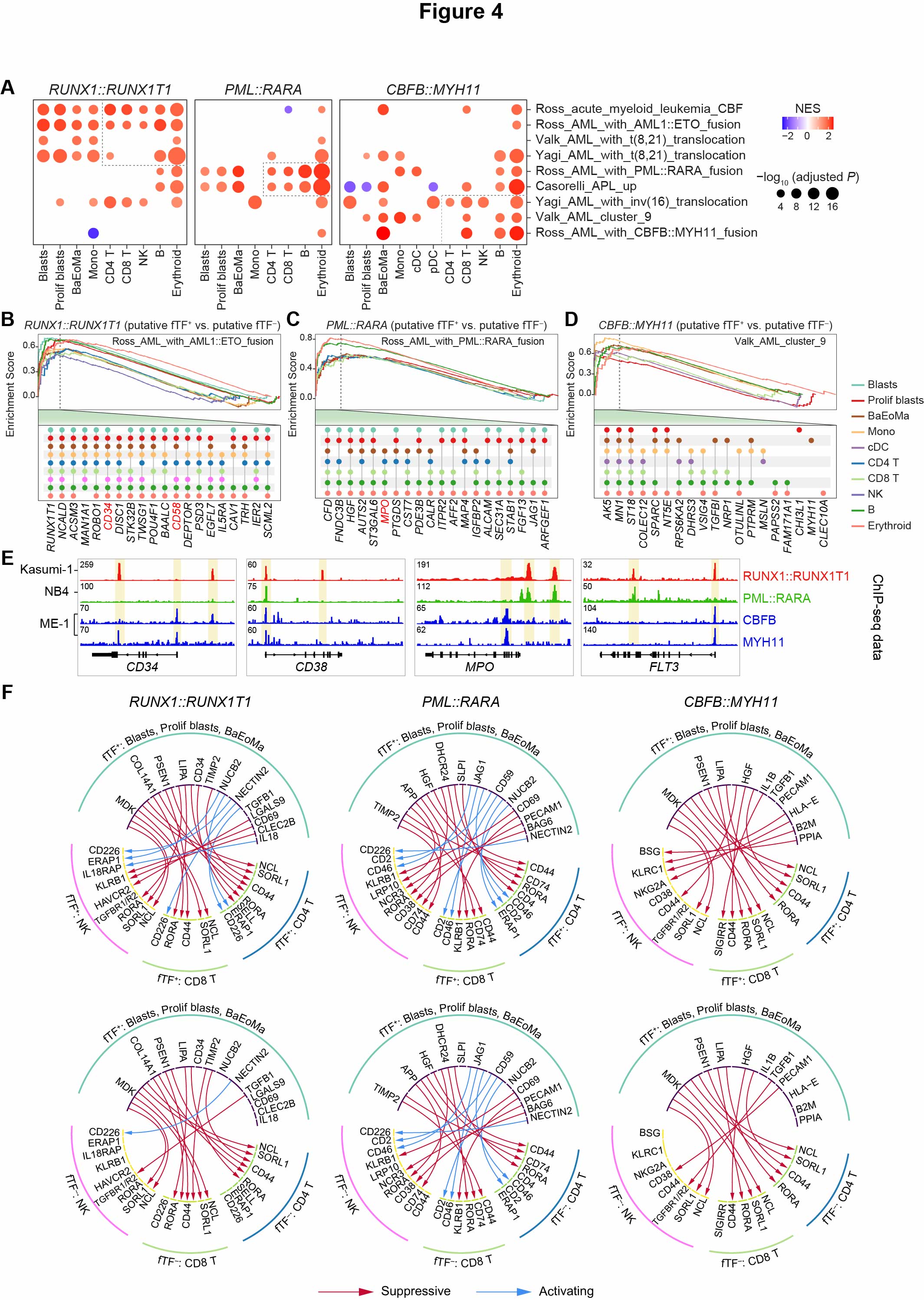 Fig. 4. Fusion transcription factors contribute to cross-lineage transcriptional aberrations in each AML subtype
(A) Dot plots showing the results of GSEA analysis using differentially expressed genes (DEGs) between putative fTF+ and fTF- cells across 11 broad cell types in RUNX1::RUNX1T1, PML::RARA, and CBFB::MYH11 AML BMs. Significantly enriched gene set terms are shown, with dashed boxes highlighting key terms across T/NK, B, and erythroid cells. (B-D) GSEA plots show that in various cell types of RUNX1::RUNX1T1 AML (B), PML::RARA AML (C), and CBFB::MYH11 AML (D), respectively, DEGs between putative fTF+ and fTF- cells are significantly enriched among the target genes of RUNX1::RUNX1T1, PML::RARA, and CBFB::MYH11. The top 20 leading-edge genes are highlighted at the bottom of each plot. (E) IGV tracks for selected gene loci, showcasing distinct ChIP-seq profiles for antibodies targeting the fusion peptide of RUNX1::RUNX1T1 (red), PML::RARA (green), and different modalities of CBFB::MYH11 (blue). (F) Circle plots of the predicted ligand-receptor interactions between putative fTF+ blasts (blasts, proliferating blasts, and BaEoMa) and immune lymphocytes across RUNX1::RUNX1T1, PML::RARA, and CBFB::MYH11 AML subtypes. The top panel shows interactions involving fTF+ CD4 T, CD8 T, and NK cells, while the bottom panel depicts interactions with fTF- immune lymphocytes. Red and blue arcs represent suppressive and activating interactions, respectively.
4.1 (A) Dot plots of GSEA results
idx.sel <- c(
    "ROSS_ACUTE_MYELOID_LEUKEMIA_CBF",
    "ROSS_AML_WITH_AML1_ETO_FUSION",
    "VALK_AML_WITH_T_8_21_TRANSLOCATION",
    "YAGI_AML_WITH_T_8_21_TRANSLOCATION",
    "ROSS_AML_WITH_PML_RARA_FUSION",
    "CASORELLI_ACUTE_PROMYELOCYTIC_LEUKEMIA_UP",
    "YAGI_AML_WITH_INV_16_TRANSLOCATION",
    "VALK_AML_CLUSTER_9",
    "ROSS_AML_WITH_CBFB_MYH11_FUSION")

res_gsea <- read_rds(paste0(in_dir, "1.10.2.degs.scAML.sub_compare_gsea.1.HC2.rds"))

df <- rbindlist(res_gsea) %>%
          filter(ID %in% idx.sel) %>%
          filter(qvalue < 0.05) %>%
          separate(group, c("FAB", "cluster"), sep = ":") %>%
          mutate(cluster = factor(cluster, levels = my_g)) %>%
          mutate(LGP = -log10(qvalue))

pdf(paste0(out_dir, "Fig4A.pdf"), width = 9.5, height = 0.21*length(idx.sel) + 1)
df %>%
  mutate(NES = Seurat::MinMax(NES, -2.5, 2.5)) %>%
  ggplot(aes_string(x = "cluster", y = "Description", size = "LGP", color = "NES")) +
    geom_point() +
    scale_y_discrete(position = "right") +
    scale_color_gradient2(low = "blue", mid = "white", high = "red", name = "Normalized \nenrichment score",
                          limits = c(-2.5, 2.5)) +
    scale_size(name = "-log10 (adj P-value)", range = c(1.5, 5)) +
    facet_grid(~ FAB, scales = "free", space = "free") +
    xlab(NULL) + ylab(NULL) + DOSE::theme_dose(8) + theme(legend.key.size = unit(0.3, "cm")) +
    theme(
      panel.grid = element_blank(),
      axis.text.x = element_text(angle = 90, hjust = 1, vjust = 0.5))
dev.off()
4.2 (B-D) GSEA plots across AML subtypes
anno_color <- c("#73C8B4", "#E31A1C", "#A65628", "#FDBF6F", "#9970AB", "#C2A5CF", "#1F78B4", "#B2DF8A", "#7570B3", "#33A02C", "#FB8072")
my_g <- c("Progs", "Progs_Prolif", "Progs_BaEoMa", "Mono", "cDC", "pDC", "CD4T", "CD8T", "NK", "B", "Erythroid")


dat_degs <- read.xlsx(paste0(in_dir, "1.10.1.degs.scAML.sub_compare.xlsx")) %>%
  mutate(group = factor(group, levels = my_g),
         cluster = factor(cluster, levels = c("M2AE", "M3PR", "M4CM")))

m2_gsdat_list <- list()
m2_gsplot_list <- list()
for(k in my_g[c(1:4, 7:11)]){
  m2_res_gsea <- run_gsea_term(dat_degs %>% filter(cluster %in% "M2AE" & group %in% k),
                           ix_path = "ROSS_AML_WITH_AML1_ETO_FUSION")
  m2_gsdat_list[[k]] <- gsInfo(m2_res_gsea, 1) %>% mutate(Description = k)
  m2_gsplot_list[[k]] <- run_gsea_plot_v2(res = m2_res_gsea, my_title = k)
}

m3_idx <- c(1:4, 7:11)
m3_gsdat_list <- list()
m3_gsplot_list <- list()
for(k in my_g[c(1:4, 7:11)]){
  m3_res_gsea <- run_gsea_term(dat_degs %>% filter(cluster %in% "M3PR" & group %in% k),
                           ix_path = "ROSS_AML_WITH_PML_RARA_FUSION")
  m3_gsdat_list[[k]] <- gsInfo(m3_res_gsea, 1) %>% mutate(Description = k)
  m3_gsplot_list[[k]] <- run_gsea_plot_v2(res = m3_res_gsea, my_title = k)
}

m4_gsdat_list <- list()
m4_gsplot_list <- list()
for(k in my_g[m4_idx]){
  m4_res_gsea <- run_gsea_term(dat_degs %>% filter(cluster %in% "M4CM" & group %in% k),
                           ix_path = "VALK_AML_CLUSTER_9")
  m4_gsdat_list[[k]] <- gsInfo(m4_res_gsea, 1) %>% mutate(Description = k)
  m4_gsplot_list[[k]] <- run_gsea_plot_v2(res = m4_res_gsea, my_title = k)
}

m2_idx <- c(1:4, 7:11)
p1_a <- my_gseaplot2(rbindlist(m2_gsdat_list) %>%
               filter(Description %in% my_g[m2_idx]) %>%
               mutate(Description = factor(Description, levels = my_g[m2_idx])),
             title = "M2\nROSS_AML_WITH_AML1_ETO_FUSION",
             rel_heights = c(1, 0.5), subplots = 1:2, base_size = 10,
             color = anno_color[m2_idx])

m3_idx <- c(1:3, 7:8, 10:11)
p1_b <- my_gseaplot2(rbindlist(m3_gsdat_list) %>%
                filter(Description %in% my_g[m3_idx]) %>%
                mutate(Description = factor(Description, levels = my_g[m3_idx])),
             title = "M3\nROSS_AML_WITH_PML_RARA_FUSION",
             rel_heights = c(1, 0.5), subplots = 1:2, base_size = 10,
             color = anno_color[m3_idx])

m4_idx <- c(2:5, 8, 10:11)
p1_c <- my_gseaplot2(rbindlist(m4_gsdat_list) %>%
               filter(Description %in% my_g[m4_idx]) %>%
               mutate(Description = factor(Description, levels = my_g[m4_idx])),
             title = "M4\nVALK_AML_CLUSTER_9",
             rel_heights = c(1, 0.5), subplots = 1:2, base_size = 10,
             color = anno_color[m4_idx])

pdf(paste0(out_dir, "Fig4B-D.pdf"), width = 12, height = 4)
wrap_plots(list(p1_a, p1_b, p1_c))
dev.off()
4.3 (F) Circle plots
g_name <- list(M2 = c("M2AE.M_M", "M2AE.M_U"),
               M3 = c("M3PR.M_M", "M3PR.M_U"),
               M4 = c("M4CM.M_M", "M4CM.M_U"))

for (i in 1:3){
  g = g_name[[i]]

  connect <- read.xlsx(paste0(in_dir, "Table.cellchat.lr_order.xlsx"), sheet = 1) %>%
    filter(!type %in% "unknown") %>%
    filter(!is.na(eval(parse(text = g[1]))) | !is.na(eval(parse(text = g[2])))) %>%
    dplyr::select(ligand, receptor, color) %>% distinct()

  g_len1 <- read.xlsx(paste0(in_dir, "Table.cellchat.lr_order.xlsx"), sheet = 1) %>%
    filter(!type %in% "unknown") %>%
    filter(!is.na(eval(parse(text = g[1]))) | !is.na(eval(parse(text = g[2])))) %>% pull(ligand_2) %>% unique() %>% length()
  g_len2 <- read.xlsx(paste0(in_dir, "Table.cellchat.lr_order.xlsx"), sheet = 1) %>%
    filter(!type %in% "unknown") %>%
    filter(!is.na(eval(parse(text = g[1]))) | !is.na(eval(parse(text = g[2])))) %>% filter(target %in% "CD4T") %>% pull(receptor_2) %>% unique() %>% length()
  g_len3 <- read.xlsx(paste0(in_dir, "Table.cellchat.lr_order.xlsx"), sheet = 1) %>%
    filter(!type %in% "unknown") %>%
    filter(!is.na(eval(parse(text = g[1]))) | !is.na(eval(parse(text = g[2])))) %>% filter(target %in% "CD8T") %>% pull(receptor_2) %>% unique() %>% length()
  g_len4 <- read.xlsx(paste0(in_dir, "Table.cellchat.lr_order.xlsx"), sheet = 1) %>%
    filter(!type %in% "unknown") %>%
    filter(!is.na(eval(parse(text = g[1]))) | !is.na(eval(parse(text = g[2])))) %>% filter(target %in% "NK") %>% pull(receptor_2) %>% unique() %>% length()

  for(j in 1:2){
    arr.col = read.xlsx(paste0(in_dir, "Table.cellchat.lr_order.xlsx")) %>%
      filter(!type %in% "unknown") %>%
      filter(!is.na(eval(parse(text = g[1]))) | !is.na(eval(parse(text = g[2])))) %>%
      mutate(color = ifelse(!is.na(eval(parse(text = g[j]))), color, adjustcolor("white", alpha.f = 0))) %>%
      dplyr::select(ligand, receptor, color) %>% distinct()


    pdf(paste0(out_dir, "Fig4F.", i, ".LR", j, ".pdf"), width = 4, height = 4)
    # parameters
    circos.clear()
    circos.par(start.degree = 160,
               gap.after = c(rep(1, g_len1 - 1), 16, rep(1, g_len2 - 1), 8, rep(1, g_len3 - 1), 8, rep(1, g_len4 - 1), 16),
               track.margin = c(-0.3, 0.3), points.overflow.warning = F)
    par(mar = c(0, 0, 0, 0))

    # color palette
    k <- length(unique(c(connect$ligand, connect$receptor)))
    n <- length(unique(connect$ligand)) + 1

    # mycolor <- viridisLite::viridis(n, alpha = 1, begin = 0, end = 1, option = "D")
    # mycolor <- c(mycolor[1:n-1], rep(mycolor[n], k-n+1))

    mycolor <- rep(c("#440154", "#8FD744", "#C7E020", "#FDE725"), c(g_len1, g_len2, g_len3, g_len4))


    myorder <- c(connect$ligand, connect$receptor) %>% unique()


    # Base plot
    chordDiagram(x = connect[, 1:3], grid.col = mycolor, col = c("white"),
                 order = myorder,
                 transparency = 0.9,
                 directional = 1, direction.type = c("arrows", "diffHeight"), diffHeight = -0.02,
                 annotationTrack = "grid", annotationTrackHeight = c(0.01, 0.1),
                 # link.arr.type = "big.arrow",
                 link.arr.length = 0.2,
                 link.arr.col = arr.col,
                 link.sort = T, link.largest.ontop = T,
                 preAllocateTracks = list(track.height = mm_h(2), track.margin = c(mm_h(2), 0))
                 )
    # Add text and axis
    circos.trackPlotRegion(
      track.index = 1, bg.border = NA,
      panel.fun = function(x, y) {
        xlim = get.cell.meta.data("xlim")
        ylim = get.cell.meta.data("ylim")
        sector.index = get.cell.meta.data("sector.index")

        # Add names to the sector.
        circos.text(x = mean(xlim) + 0.25, y = -8, adj = -0.05,
                    labels = sector.index, facing = "clockwise", cex = 0.7, niceFacing = T)

        # # Add graduation on axis
        # circos.axis(
        #   h = "top", major.at = seq(ligand = 0, to = xlim[2],
        #                             by = ifelse(test = xlim[2] > 10, yes = 2, no = 1)),
        #   minor.ticks = 1, major.tick.percentage = 0.5, labels.niceFacing = FALSE)
      }
    )

    ## # Add group info
    brand <- setNames(unlist(lapply(myorder, function(x) unlist(str_split(x, "_"))[1])), myorder)
    brand_color <-setNames(c("#73C8B4", "#1F78B4", "#B2DF8A", "#FF77F8"), c("Progs", "CD4T", "CD8T", "NK"))

    for(b in unique(brand)) {
      model = names(brand[brand == b])
      highlight.sector(sector.index = model, track.index = 1, col = brand_color[b], padding = c(-0.7, 0, 0, 0),
                       text = b, text.vjust = -0.5, niceFacing = TRUE)
    }

    dev.off()
  }
}