5 Figure 5
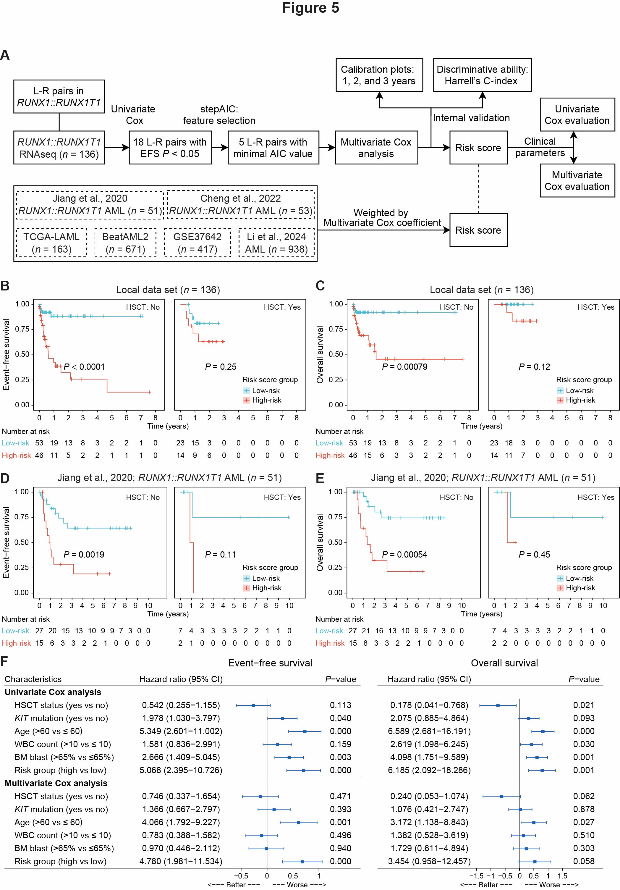 Fig.5. Construction of a prognostic risk model based on intercellular communications in RUNX1::RUNX1T1 AML
(A) Workflow diagram illustrating the process for generating RUNX1::RUNX1T1 AML-specific L-R pair risk scores and their validation using publicly available datasets. (B-C) Kaplan–Meier curve for EFS (B) and OS (C) stratified by HSCT status, based on risk score groups in 136 local RUNX1::RUNX1T1 AML cases. P-value was calculated using the log-rank test. (D-E) Kaplan–Meier curve for EFS (D) and OS (E) stratified by HSCT status, based on risk score groups in the external validation dataset by Jiang et al. (51 RUNX1::RUNX1T1 AML cases, non-overlapping with our local dataset). P-value was calculated using the log-rank test. (F) Forest plot of univariate and multivariate Cox regression analyses incorporating traditional clinical parameters and risk score groups. Hazard ratios and 95% CIs are displayed alongside each variable, with the x-axis on a \(log_{10}\)(HR) scale. In the forest plot, HRs are represented by boxes, while horizontal lines depict the 95% CIs. The vertical line at \(log_{10}\)(HR) = 0 (HR = 1) indicates no statistically significant effect, while values to the right of this line (HR > 1) suggest worse outcomes. P-values were calculated using the Wald test.
5.1 (B-C) KM plot of local data
fit <- survfit(Surv(OS_days, OS_status) ~ Risk_score_g + HSCT, data = dat_clin)
OS_combine1 <- ggsurvplot_facet(fit, data = dat_clin, facet.by = "HSCT", palette = g_color, title = "OS",
                                pval = T, conf.int = T, break.time.by = 365)
OS_combine2 <- ggsurvplot(fit, data = dat_clin, risk.table = T, break.time.by = 365)

fit <- survfit(Surv(EFS_days, EFS_status) ~  Risk_score_g + HSCT, data = dat_clin)
EFS_combine1 <- ggsurvplot_facet(fit, data = dat_clin, facet.by = "HSCT", palette = g_color, title = "EFS",
                                pval = T, conf.int = T, break.time.by = 365)
EFS_combine2 <- ggsurvplot(fit, data = dat_clin, risk.table = T, break.time.by = 365)


pdf(paste0(out_dir, "Fig5B-C.pdf"), width = 18, height = 7.5)
ggarrange(EFS_combine1, OS_combine1,
          EFS_combine2$table + facet_wrap(. ~ HSCT, scales = "free") +
              theme(legend.position = "none", strip.text.x = element_blank()) +
              scale_y_discrete(labels = rev(c("Low", "High"))),
          OS_combine2$table + facet_wrap(. ~ HSCT, scales = "free") +
              theme(legend.position = "none", strip.text.x = element_blank()) +
              scale_y_discrete(labels = rev(c("Low", "High"))),
          labels = NULL, ncol=2, nrow=2, font.label = list(size = 10), align = "hv",
          heights = c(1, 0.5))
dev.off()
5.2 (D-E) KM plot of local data
fit <- survfit(Surv(OS_days, OS_status) ~ Risk_score_g + HSCT, data = pnas_clin)
OS_combine1 <- ggsurvplot_facet(fit, data = pnas_clin, facet.by = "HSCT", palette = g_color, title = "OS",
                                pval = T, conf.int = T, break.time.by = 365)
OS_combine2 <- ggsurvplot(fit, data = pnas_clin, risk.table = T, break.time.by = 365)

fit <- survfit(Surv(EFS_days, EFS_status) ~  Risk_score_g + HSCT, data = pnas_clin)
EFS_combine1 <- ggsurvplot_facet(fit, data = pnas_clin, facet.by = "HSCT", palette = g_color, title = "EFS",
                                pval = T, conf.int = T, break.time.by = 365)
EFS_combine2 <- ggsurvplot(fit, data = pnas_clin, risk.table = T, break.time.by = 365)


pdf(paste0(out_dir, "Fig5D-E.pdf"), width = 18, height = 7.5)
ggarrange(EFS_combine1, OS_combine1,
          EFS_combine2$table + facet_wrap(. ~ HSCT, scales = "free") +
              theme(legend.position = "none", strip.text.x = element_blank()) +
              scale_y_discrete(labels = rev(c("Low", "High"))),
          OS_combine2$table + facet_wrap(. ~ HSCT, scales = "free") +
              theme(legend.position = "none", strip.text.x = element_blank()) +
              scale_y_discrete(labels = rev(c("Low", "High"))),
          labels = NULL, ncol=2, nrow=2, font.label = list(size = 10), align = "hv",
          heights = c(1, 0.5))
dev.off()
5.3 (F) Forest plot of EFS and OS
# OS
d <- cbind(Characteristics = c(NA, "Univariate Cox analysis", rownames(AE_comb_uni_cox_OS),
                               "Multivariate Cox analysis", rownames(AE_comb_multi_cox_OS)),
           rbind(NA, NA, AE_comb_uni_cox_OS, NA, AE_comb_multi_cox_OS))
d$Characteristics <- as.character(d$Characteristics)
hr_info_OS <- d %>% dplyr::select(mean = `exp(coef)`, lower = `lower .95`, upper = `upper .95`) %>%
  mutate_if(is.character, as.numeric)
tabletext_OS <- d[, c("Characteristics", "HR.interval", "Pr(>|z|)")]
tabletext_OS[1, ] <- c("Characteristics", "Hazard ratio (95% CI)", "P-value")

# EFS
d <- cbind(Characteristics = c(NA, "Univariate Cox analysis", rownames(AE_comb_multi_cox_EFS),
                               "Multivariate Cox analysis", rownames(AE_comb_multi_cox_EFS)),
           rbind(NA, NA, AE_comb_uni_cox_EFS, NA, AE_comb_multi_cox_EFS))
d$Characteristics <- as.character(d$Characteristics)
hr_info_EFS <- d %>% dplyr::select(mean = `exp(coef)`, lower = `lower .95`, upper = `upper .95`) %>%
  mutate_if(is.character, as.numeric)
tabletext_EFS <- d[, c("Characteristics", "HR.interval", "Pr(>|z|)")]
tabletext_EFS[1, ] <- c("Characteristics", "Hazard ratio (95% CI)", "P-value")


pdf(paste0(out_dir, "Fig5F.pdf"), width = 15, height = 5.5, useDingbats = F)
library(grid)
grid.newpage()
borderWidth <- unit(1, "pt")
width <- unit(convertX(unit(1, "npc") - borderWidth, unitTo = "npc", valueOnly = TRUE)/3, "npc")
pushViewport(viewport(layout = grid.layout(nrow = 1, ncol = 3,
                                           widths = unit.c(width*1.7, borderWidth, width, borderWidth, width))))

pushViewport(viewport(layout.pos.row = 1, layout.pos.col = 1))
forestplot(labeltext = tabletext_EFS, hr_info_EFS, title = "Event–free survival",
           xlab="<--- Better ---      --- Worse --->",
           hrzl_lines = list("2" = gpar(lwd = 1), "9" = gpar(lwd = 1)), clip = c(0, 3),
           graph.pos = 3, graphwidth = unit(5, "cm"),
           col=fpColors(box = "#1c61b6", lines = "#1c61b6", zero = "gray50"),
           zero = 1, cex = 0.9, lineheight = "auto", colgap = unit(6, "mm"), lwd.ci = 2,
           boxsize = 0.2, ci.vertices = T, ci.vertices.height = 0.1,
           new_page = FALSE)
upViewport()

pushViewport(viewport(layout.pos.row = 1, layout.pos.col = 2))
grid.rect(gp = gpar(fill = "#FFFFFF", col = "#eeeeee"))
upViewport()

pushViewport(viewport(layout.pos.row = 1, layout.pos.col = 3))
forestplot(labeltext = tabletext_OS[, 2:3], hr_info_OS, title = "Overall survival",
           xlab="<--- Better ---      --- Worse --->",
           hrzl_lines = list("2" = gpar(lwd = 1), "9" = gpar(lwd = 1)), clip = c(0, 3),
           graph.pos = 2, graphwidth = unit(5, "cm"),
           col=fpColors(box = "#1c61b6", lines = "#1c61b6", zero = "gray50"),
           zero = 1, cex = 0.9, lineheight = "auto", colgap = unit(6, "mm"), lwd.ci = 2,
           boxsize = 0.2, ci.vertices = T, ci.vertices.height = 0.1,
           new_page = FALSE)

upViewport()
dev.off()