2 Figure 2

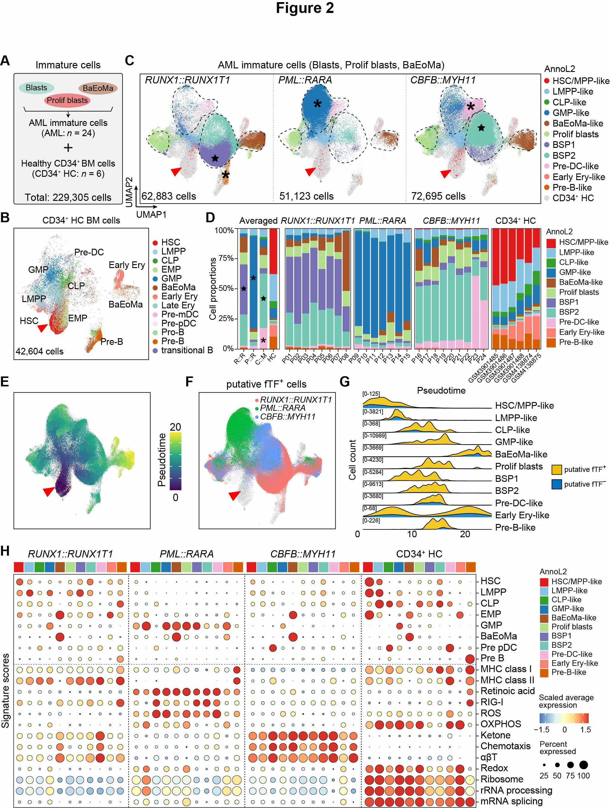Fig. 2. Differentiation hierarchies of leukemic blasts across different AML subtypes

(A) Illustration of merged analysis of blasts in AML BM samples, utilizing 6 publicly available CD34⁺ BMMCs as healthy controls (HC).
(B) UMAP visualization of public CD34⁺ HC cells, with colors indicating Azimuth level 2 annotations of hematopoietic cell types. The total number of sequenced cells is indicated in the bottom-left corner. The red arrowhead indicates the HSC population.
(C) UMAP visualizations of cell types from RUNX1::RUNX1T1, PML::RARA, and CBFB::MYH11 AML, with colors indicating semi-supervised annotation level 2 (annoL2). Grey indicates healthy CD34⁺ HC cells. The total number of sequenced cells for each AML subtype is indicated in the bottom-left corner. The red arrowhead indicates the HSC/MPP-like population, while the dashed box, asterisk and star highlight key populations.
(D) Bar charts depicting the relative fractions of 11 annotated cell types across different groups. The left panel shows the average fractions for each group, while the other panels present individual sample fractions. Key cell populations are marked with an asterisk or star.
(E) UMAP visualization of monocle3-pseudotime scores. The red arrowhead indicates the HSC/MPP-like population.
(F) UMAP visualization showing the distribution of putative fTF⁺ cells: RUNX1::RUNX1T1 (red), PML::RARA (green), and CBFB::MYH11 (blue), with grey representing putative fTF^- cells. The red arrowhead indicates the HSC/MPP-like population. Grey indicates healthy CD34⁺ HC and putative fTF^- cells from AML samples.
(G) Distribution of cell types along the pseudotime score axis, showing only cells derived from AML patients.
(H) Dot plots of signature scores for gene sets characterizing relevant biological processes across 11 different hematopoietic cell types in AML subtypes and HC groups.
R::R, RUNX1::RUNX1T1 AML; P::R, PML::RARA AML; C::M, CBFB::MYH11 AML.

2.1 (B) UMAP of HC

scAML.prog.anno <- read_rds(paste0(in_dir, "Table1.3.scAML.prog_harmony.anno.rds"))

p2 <- DimPlot(scAML.prog.anno, reduction = "umap", group.by = "predicted.celltype.l2", split.by = "FAB", 
    pt.size = 1, label = F, repel = T, raster = T, cols = pcol_2)

pdf(paste0(out_dir, "Fig2B.pdf"), width = 20, height = 9)
p1 + p2
dev.off()

2.2 (C) UMAP distribution across AML subtypes

anno_color <- c("#E31A1C", "#86C2E2", "#33A02C", "#1F78B4", "#A65628", "#B2DF8A", "#7570B3", "#73C8B4", "#F1B6DA", "#FB8072", "#D95F02")
anno_name <- c("HSC.MPP-like", "LMPP-like", "CLP-like", "GMP-like", "BaEoMa-like", "Progs-Prolif", "NPW-high", "LSC17-high", "Pre-DC", "Erythroid", "Pre-B")


anno_color2 <- c("HC_CD34" = "#D9D9D9", anno_color)

scAML.sub1 <- scAML.prog.anno %>% subset(FAB %in% c("M2AE", "HC_CD34"))
scAML.sub1@meta.data <- scAML.sub1@meta.data %>% 
    mutate(annoL2 = as.character(annoL2), 
           annoL2 = ifelse(FAB %in% "HC_CD34", "HC_CD34", annoL2),
           annoL2 = factor(annoL2, levels = names(anno_color2)[c(1:2, 4:5, 3, 6:7, 10:12, 9, 8)]))
p1 <- DimPlot(scAML.sub1, reduction = "umap", group.by = "annoL2", cols = anno_color2,
        order = T, label = F, repel = T, raster = T, pt.size = 0.5) + labs(title = "M2")

scAML.sub2 <- scAML.prog.anno %>% subset(FAB %in% c("M3PR", "HC_CD34"))
scAML.sub2@meta.data <- scAML.sub2@meta.data %>% 
    mutate(annoL2 = as.character(annoL2), 
           annoL2 = ifelse(FAB %in% "HC_CD34", "HC_CD34", annoL2),
           annoL2 = factor(annoL2, levels = names(anno_color2)[c(1:2, 4, 6:12, 5, 3)]))
p2 <- DimPlot(scAML.sub2, reduction = "umap", group.by = "annoL2", cols = anno_color2,
        order = T, label = F, repel = T, raster = T, pt.size = 0.5) + labs(title = "M3")

scAML.sub3 <- scAML.prog.anno %>% subset(FAB %in% c("M4CM", "HC_CD34"))
scAML.sub3@meta.data <- scAML.sub3@meta.data %>% 
    mutate(annoL2 = as.character(annoL2), 
           annoL2 = ifelse(FAB %in% "HC_CD34", "HC_CD34", annoL2),
           annoL2 = factor(annoL2, levels = names(anno_color2)[c(1:2, 4:7, 10:12, 3, 8:9)]))
p3 <- DimPlot(scAML.sub3, reduction = "umap", group.by = "annoL2", cols = anno_color2,
        order = T, label = F, repel = T, raster = T, pt.size = 0.5) + labs(title = "M4")


pdf(paste0(out_dir, "Fig2C.pdf"), width = 13, height = 4)
p1 + p2 + p3 + plot_layout(ncol = 3, guides = "collect")
dev.off()

2.3 (D) Bar charts

p1 <- plot_stat(scAML.prog.anno, plot_type = "prop_fill", group_by = "FAB", pal_setup = anno_color) + 
    theme(axis.text.x = element_text(angle = 45, hjust = 1, vjust = 1))
p2 <- plot_stat(scAML.prog.anno, plot_type = "prop_fill", group_by = "orig.ident", pal_setup = anno_color) + 
    theme(axis.text.x = element_text(angle = 45, hjust = 1, vjust = 1))

pdf(paste0(out_dir, "Fig2D.pdf"), width = 9,  height = 4)
p1 + p2 + plot_layout(ncol = 2, widths = c(0.45, 3), guides = "collect")
dev.off()

2.4 (E) Pseudotime UMAP

cds <- read_rds(paste0(in_dir, "Table1.4.scAML.prog_harmony.anno.monocle3.rds"))

scAML.prog.anno <- AddMetaData(object = scAML.prog.anno, 
    metadata = cds@principal_graph_aux@listData$UMAP$pseudotime, col.name = "pseudotime")

pdf(paste0(out_dir, "Fig2E.pdf"), width = 4, height = 3.5)
FeaturePlot(scAML.prog.anno, features = "pseudotime", pt.size = 0.4, order = T, reduction = "umap", raster = T)  & 
            scale_color_viridis_c()
dev.off()

2.5 (F) Putative fTF-expression cells distribution

res_pred <- read_rds(paste0(in_dir, "Table1.res_pred.351594.rds")) %>%
    rownames_to_column("ID") %>% dplyr::select(ID, SS.final_fus_group)

df <- scAML.prog.anno@meta.data %>%
        rownames_to_column("ID") %>% 
        left_join(., res_pred) %>% 
        mutate(fus_group2 = case_when(
            (SS.final_fus_group == "Malignant" & FAB == "M2AE") ~ "M2AE",
            (SS.final_fus_group == "Malignant" & FAB == "M3PR") ~ "M3PR",
            (SS.final_fus_group == "Malignant" & FAB == "M4CM") ~ "M4CM",
            (SS.final_fus_group == "Unclear") ~ "ANA")) %>% 
        left_join(., scAML.prog.anno@reductions$umap@cell.embeddings %>% data.frame() %>% rownames_to_column("ID")) %>% 
            column_to_rownames("ID")

df1 <- df %>% filter(SS.final_fus_group == "Unclear")
df2 <- df %>% filter(SS.final_fus_group != "Unclear") %>% sample_n(nrow(.))
pdf(paste0(out_dir, "Fig2F.pdf"), width = 4.7, height = 3.5)
rbind(df1, df2) %>% 
    mutate(mysize = ifelse((SS.final_fus_group == "Unclear"), 1, 2)) %>%
ggplot() + 
  ggrastr::rasterise(geom_point(aes_string(x = "umap_1", y = "umap_2", color = "fus_group2", size = "mysize"), 
        stroke = 0, alpha = 1), dpi = 300) + 
  scale_color_manual(values = c("#D9D9D9", "#F8766D", "#00BA38", "#619CFF")) + 
  scale_size_continuous(range = c(0.05, 0.2)) + 
  ggthemes::theme_few()
dev.off()

2.6 (G) Ridge plot of pseudotime

cds <- read_rds(paste0(in_dir, "Table1.4.scAML.prog_harmony.anno.monocle3.rds"))

scAML.prog.anno <- AddMetaData(object = scAML.prog.anno, 
    metadata = cds@principal_graph_aux@listData$UMAP$pseudotime, col.name = "pseudotime")

df <- scAML.prog.anno@meta.data %>% rownames_to_column("ID") %>% 
        left_join(., scAML.prog.anno@reductions$umap@cell.embeddings %>% data.frame() %>% rownames_to_column("ID")) %>% 
        left_join(., res_pred) %>% 
        column_to_rownames("ID")

pdf(paste0(out_dir, "Fig2G.pdf"), width = 7, height = 4, useDingbats = F)
df %>% 
ggplot(aes(x = pseudotime, fill = SS.final_fus_group)) +
  geom_density(alpha = 0.9, adjust = 1.2, trim = F, position = "stack") +
  scale_fill_manual(values = c("Malignant" = "#EFC000", "Unclear" = "#0073C2")) +
  theme_minimal() +
  facet_grid(annoL2 ~ ., scales = "free") + 
  theme(panel.grid = element_blank(), 
        panel.spacing = unit(0, "lines"),
        strip.text.y = element_text(angle = 0, hjust = 0),
        axis.text.y = element_blank(), axis.ticks.y = element_blank()
        )
dev.off()

2.7 (H) Dot plots of signature scores

idx_feature = rev(colnames(scAML.prog.anno@meta.data)[c(25:37, 40:58)])
p <- DotPlot(object = scAML.prog.anno, assay = "RNA", features = idx_feature, cols = "RdYlBu", 
        group.by = "FAB", split.by = "annoL2") + 
        geom_point(aes(size = pct.exp), shape = 21, stroke = 0.2) + 
        theme_bw() + theme(axis.text.x = element_text(angle = 90, hjust = 1, vjust = 0.5)) + coord_flip()

anno_name <- c("HSC.MPP-like", "LMPP-like", "CLP-like", "GMP-like", "BaEoMa-like", "Progs-Prolif", "NPW-high", "LSC17-high", "Pre-DC", "Erythroid", "Pre-B")
df_raw <- p$data %>% 
                mutate(FAB = str_extract(id, "M2AE|M3PR|M4CM|HC_CD34"), 
                       annoL2 = str_replace_all(id, "M2AE_|M3PR_|M4CM_|HC_CD34_", "")) %>% 
                mutate(FAB = factor(FAB, levels = c("M2AE", "M3PR", "M4CM", "HC_CD34")),
                       annoL2 = factor(annoL2, levels = anno_name))
p1 <- df_raw %>% 
        group_by(features.plot) %>% 
        mutate(avg.exp.scaled = MinMax(avg.exp.scaled, -1.5, 1.5)) %>%
    ggplot() + 
        geom_point(aes(x = id, y = features.plot, fill = avg.exp.scaled, size = pct.exp), shape = 21, stroke = 0) + 
        facet_grid(~FAB, scales = "free", space = "free") + 
        scale_fill_distiller(palette ="RdYlBu") + 
    theme_bw() + theme(axis.text.x = element_text(angle = 90, hjust = 1, vjust = 0.5)) + 
    scale_radius(range = c(0, 6))

pdf(paste0(out_dir, "Fig2H.pdf"), width = 12, height = 9)
p1
dev.off()